
| Research History |
| Software Structure |
| Specie Sensitivity Distribution |
| BAYESIAN Inference |
| MCMC Simulation |
| DIC Optimization |
| Ecorisk & Uncertainty |
| Joint Probability Curve |
| Exergy SSD |
| Main Function Lists |
| BMC-SSD Interface |
| Models Optimization |
| JPC interface |
| ExSSD interface |
| Work Path & Output Results |
| Installation & Initialization |
| Folder & File Extraction |
| SSD Models & Ecorisk |
| JPC & Its Indicators |
| Models Optimization & Parameters |
| ExSSD Models & ExEcorisk |
Links
| College of Urban and Environment Science |
| Peking University |
SSD models
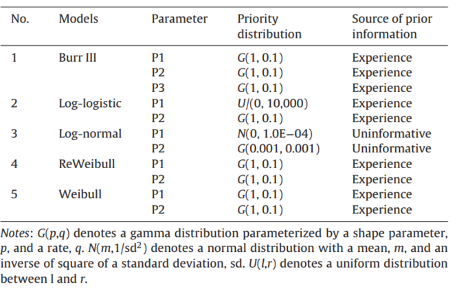
Our BMC-SSD platform have 9 built-in SSD models. However, considering both toxicity and exposure data are nonnegative, Normal,Logistic,Burr II models are meaningless since their inverse functions can result in negative risks during calculation, therefore, only 5 out of 9 SSD models are suitable for the nonnegative limitation (Burr III, Log-logistic, Log-normal, ReWeibull and Weibull). Among the models, Log-logistic and Log-normal are most commonly used in SSD model building (Solomon et al., 1996; Newman et al., 2000; Solomon et al., 2000; Fisher and Burton, 2003; Wang et al., 2010), while Burr III and its special situation ReWeibull are first introduced by Shao (2000). Before establishing SSD models, there are two crucial steps. First is to calculate cumulative probability by the formula PR = R / (N + 1), where R is rank of the toxicity or exposure data order of a certain chemical, and N represents the total number of species. The second step is to use statistical methods like Least Square Method or Maximum Likelihood Score or Bayesian Simulation to simulate the parameters of SSD models (Solomon et al., 2000; Hose and Van den Brink, 2004; Grist et al., 2006). For the SSD curves, the x-axis represents toxicity or exposure data with the unit of ng/L or μg/L while the y-axis represents probability value. When building SSD model, the cumulative distribution functions (CDF) of the above models are applied while the inverse functions of the CDF (CDF-1) are used when the corresponding concentrations are needed for defined risks. The CDF and CDF-1 of the five models are shown in Table 1. For the prior selection of SSD model parameters, WinBUGS is applied to calculate posterior distribution of the parameters. According to preliminary tests, all the parameters in SSD models are positive numbers, and their prior distributions all follow gamma distribution except for P1 in Log-normal model (as P1 is real number, it follows normal distribution). The prior distributions of all models are shown in Table 2.
Table 1 SSD models' cummulative probability fnction (CDF) and its inverse function CDF-1

Table 2 Priority distribution of the parameters in five SSD models
![]()